Introduction

In this notebook, We will conduct a very basic attempt at topic modelling this Spooky Author dataset (Kaggle). Topic modelling is the process in which we try uncover abstract themes or “topics” based on the underlying documents and words in a corpus of text. We will introduce standard topic modelling techniques known as Latent Dirichlet Allocation (LDA).
The outline of this notebook is as follows:
-
Exploratory Data Analysis (EDA) and WordClouds - Analyzing the data by generating simple statistics such word frequencies over the different authors as well as plotting some wordclouds (with image masks).
-
Topic Modelling with LDA - Implementing the topic modelling technique using Scikit-Learn : Latent Dirichlet Allocation (LDA)
import base64
import numpy as np
import pandas as pd

# NLtk
import nltk
from nltk.stem import WordNetLemmatizer


# Plotly imports
import plotly.offline as py
py.init_notebook_mode(connected=True)
import plotly.graph_objs as go
import plotly.tools as tls

# Other imports
from collections import Counter
from sklearn.feature_extraction.text import TfidfVectorizer, CountVectorizer
from sklearn.decomposition import NMF, LatentDirichletAllocation
from matplotlib import pyplot as plt
%matplotlib inline
# Loading in the training data with Pandas
train = pd.read_csv("./data/spooky_authors.csv")
1. The Authors and their works EDA
First step, let us take a look at a quick peek of what the first three rows in the data has in store for us and who exactly are the authors
train.head()
| id | text | author | |
|---|---|---|---|
| 0 | id26305 | This process, however, afforded me no means of... | EAP |
| 1 | id17569 | It never once occurred to me that the fumbling... | HPL |
| 2 | id11008 | In his left hand was a gold snuff box, from wh... | EAP |
| 3 | id27763 | How lovely is spring As we looked from Windsor... | MWS |
| 4 | id12958 | Finding nothing else, not even gold, the Super... | HPL |
According to the competition page there are three distinct author initials we have already been provided with a mapping of these initials to the actual author which is as follows:
(Links to their Wikipedia page profiles if you click on their names)
-
EAP - Edgar Allen Poe : American writer who wrote poetry and short stories that revolved around tales of mystery and the grisly and the grim. Arguably his most famous work is the poem - “The Raven” and he is also widely considered the pioneer of the genre of the detective fiction.
-
HPL - HP Lovecraft : Best known for authoring works of horror fiction, the stories that he is most celebrated for revolve around the fictional mythology of the infamous creature “Cthulhu” - a hybrid chimera mix of Octopus head and humanoid body with wings on the back.
-
MWS - Mary Shelley : Seemed to have been involved in a whole panoply of literary pursuits - novelist, dramatist, travel-writer, biographer. She is most celebrated for the classic tale of Frankenstein where the scientist Frankenstein a.k.a “The Modern Prometheus” creates the Monster that comes to be associated with his name.
Next, let us take a look at how large the training data is:
train['author'].value_counts()
EAP    7900
MWS    6044
HPL    5635
Name: author, dtype: int64
print(train.shape)
(19579, 3) ## WordClouds to visualise each author's work
One very handy visualization tool for a data scientist when it comes to any sort of natural language processing is plotting “Word Cloud”. A word cloud (as the name suggests) is an image that is made up of a mixture of distinct words which may make up a text or book and where the size of each word is proportional to its word frequency in that text (number of times the word appears). Here instead of dealing with an actual book or text, our words can simply be taken from the column “text”
Store the text of each author in a Python list
We first create three different python lists that store the texts of Edgar Allen Poe, HP Lovecraft and Mary Shelley respectively as follows:
eap = train[train.author=="EAP"]["text"].values
hpl = train[train.author=="HPL"]["text"].values
mws = train[train.author=="MWS"]["text"].values
Next to create our wordclouds, I will import the python module “wordcloud”.
from wordcloud import WordCloud, STOPWORDS
Finally plotting the word clouds via the following few lines (unhide to see the code):
# The wordcloud of Cthulhu/squidy thing for HP Lovecraft
plt.figure(figsize=(16,13))
wc = WordCloud(background_color="black", max_words=10000,
               stopwords=STOPWORDS, max_font_size= 40)
wc.generate(" ".join(hpl))
plt.title("HP Lovecraft (Cthulhu-Squidy)", fontsize=20)
# plt.imshow(wc.recolor( colormap= 'Pastel1_r' , random_state=17), alpha=0.98)
plt.imshow(wc.recolor( colormap= 'Pastel2' , random_state=17), alpha=0.98)
plt.axis('off')
(-0.5, 399.5, 199.5, -0.5)

plt.figure(figsize=(20,18))
# The wordcloud of the raven for Edgar Allen Poe
plt.subplot(211)
wc = WordCloud(background_color="black",
               max_words=10000,
               stopwords=STOPWORDS,
               max_font_size= 40)
wc.generate(" ".join(eap))
plt.title("Edgar Allen Poe (The Raven)")
plt.imshow(wc.recolor( colormap= 'PuBu' , random_state=17), alpha=0.9)
plt.axis('off')
(-0.5, 399.5, 199.5, -0.5)

plt.figure(figsize=(20,18))
wc = WordCloud(background_color="black",
               max_words=10000,
               stopwords=STOPWORDS,
               max_font_size= 40)
wc.generate(" ".join(mws))
plt.title("Mary Shelley (Frankenstein's Monster)", fontsize= 18)
plt.imshow(wc.recolor( colormap= 'viridis' , random_state=17), alpha=0.9)
plt.axis('off')
(-0.5, 399.5, 199.5, -0.5)

Well there you have it, three separate word clouds, one for each of our spooky authors. Right off the bat, you can see from these word clouds some of the choice words that were favoured by the different authors.
For example, you can see the HP lovecraft favours words like “dream”, “time”, “strange”, “past”, “ancient” which seem to resonate with themes that the author was famous for, themes around the hidden psyche and esoteric nature of fate and chance as well as the infamous creature Cthulhu and mentions of ancient cults and rituals associated with it.
On the other hand, one can see that Mary Shelley’s words revolve around primal instincts and themes of morality which range from the positive to negative ends of the spectrum, such as “friend”, “fear”, “hope”, “spirit” etc. - themes which resonate in her works such as Frankenstein
However, as you can see from the word clouds, there are still a handful of words that seem to be quite out of place. Words such as “us”, “go”, “he” which seem to appear commonly every where in text
2. Topic modelling

What is Topic Modeling?
Topic modeling is a method for unsupervised classification of documents, similar to clustering on numeric data, which finds some natural groups of items (topics) even when we’re not sure what we’re looking for.
Why Topic Modeling?
Topic modeling provides methods for automatically organizing, understanding, searching, and summarizing large text documents. It can help with the following:
- discovering the hidden themes in the collection.
- classifying the documents into the discovered themes.
- using the classification to organize/summarize/search the documents.
For example, let’s say a document belongs to the topics food, dogs and health. So if a user queries “dog food”, they might find the above-mentioned document relevant because it covers those topics(among other topics). We are able to figure its relevance with respect to the query without even going through the entire document.
Therefore, by annotating the document, based on the topics predicted by the modeling method, we are able to optimize our search process.
Latent Dirichlet Allocation (LDA)
It is one of the most popular topic modeling methods. Each document is made up of various words, and each topic also has various words belonging to it. The aim of LDA is to find topics a document belongs to, based on the words in it. Confused much? Here is an example to walk you through it.

Model Definition
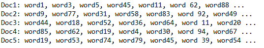
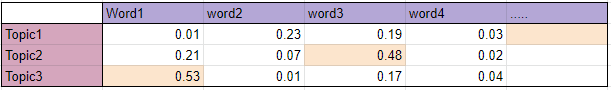
We have 5 documents each containing the words listed in front of them( ordered by frequency of occurrence). What we want to figure out are the words in different topics, as shown in the table below. Each row in the table represents a different topic and each column a different word in the corpus. Each cell contains the probability that the word(column) belongs to the topic(row).
Finding Representative Words for a Topic
- We can sort the words with respect to their probability score. The top x words are chosen from each topic to represent the topic. If x = 10, we’ll sort all the words in topic1 based on their score and take the top 10 words to represent the topic. This step may not always be necessary because if the corpus is small we can store all the words in sorted by their score.
- Alternatively, we can set a threshold on the score. All the words in a topic having a score above the threshold can be stored as its representative, in order of their scores.
Let’s say we have 2 topics that can be classified as CAT_related and DOG_related. A topic has probabilities for each word, so words such as milk, meow, and kitten, will have a higher probability in the CAT_related topic than in the DOG_related one. The DOG_related topic, likewise, will have high probabilities for words such as puppy, bark, and bone.
If we have a document containing the following sentences:
“Dogs like to chew on bones and fetch sticks”. “Puppies drink milk.” “Both like to bark.”
We can easily say it belongs to topic DOG_related because it contains words such as Dogs, bones, puppies, and bark. Even though it contains the word milk which belongs to the topic CAT_related, the document belongs to DOG_related as more words match with it.
# Define helper function to print top words
def print_top_words(model, feature_names, n_top_words):
    for index, topic in enumerate(model.components_):
        message = "\nTopic #{}:".format(index)
        message += ", ".join([feature_names[i] for i in topic.argsort()[:-n_top_words - 1 :-1]])
        print(message)
        print("="*70)
2a. Putting all the preprocessing steps together
Unfortunately, there is no built-in lemmatizer in the vectorizer so we are left with a couple of options. Either implementing it separately everytime before feeding the data for vectorizing or somehow extend the sklearn implementation to include this functionality. Luckily for us, we have the latter option where we can extend the CountVectorizer class by overwriting the “build_analyzer” method as follows:
Extending the CountVectorizer class with a lemmatizer
lemm = WordNetLemmatizer()
class LemmaCountVectorizer(CountVectorizer):
    def build_analyzer(self):
        analyzer = super(LemmaCountVectorizer, self).build_analyzer()
        return lambda doc: (lemm.lemmatize(w) for w in analyzer(doc))
Here we have utilised some subtle concepts from Object-Oriented Programming (OOP). We have essentially inherited and subclassed the original Sklearn’s CountVectorizer class and overwritten the build_analyzer method by implementing the lemmatizer for each list in the raw text matrix.
# Storing the entire training text in a list
text = list(train.text.values)
# Calling our overwritten Count vectorizer
tf_vectorizer = LemmaCountVectorizer(max_df=0.95,
                                     min_df=2,
                                     stop_words='english',
                                     decode_error='ignore')
tf = tf_vectorizer.fit_transform(text)
2b. Latent Dirichlet Allocation
Finally we arrive on the subject of topic modelling and the implementation of a couple of unsupervised learning algorithms. The first method that We will touch upon is Latent Dirichlet Allocation. Now there are a couple of different implements of this LDA algorithm but in this notebook, We will be using Sklearn’s implementation. Another very well-known LDA implementation is Radim Rehurek’s gensim, so check it out as well.
Corpus - Document - Word : Topic Generation
The LDA algorithm first models documents via a mixture model of topics. From these topics, words are then assigned weights based on the probability distribution of these topics. It is this probabilistic assignment over words that allow a user of LDA to say how likely a particular word falls into a topic. Subsequently from the collection of words assigned to a particular topic, are we thus able to gain an insight as to what that topic may actually represent from a lexical point of view.
lda = LatentDirichletAllocation(n_components=11, max_iter=5,
                                learning_method = 'online',
                                learning_offset = 50.,
                                random_state = 0)
##
lda.fit(tf)
LatentDirichletAllocation(batch_size=128, doc_topic_prior=None,
                          evaluate_every=-1, learning_decay=0.7,
                          learning_method='online', learning_offset=50.0,
                          max_doc_update_iter=100, max_iter=5,
                          mean_change_tol=0.001, n_components=11, n_jobs=None,
                          perp_tol=0.1, random_state=0, topic_word_prior=None,
                          total_samples=1000000.0, verbose=0)
Topics generated by LDA
We will utilise our helper function we defined earlier “print_top_words” to return the top 10 words attributed to each of the LDA generated topics. To select the number of topics, this is handled through the parameter n_components in the function.
n_top_words = 40
print("\nTopics in LDA model: ")
tf_feature_names = tf_vectorizer.get_feature_names()
print_top_words(lda, tf_feature_names, n_top_words)
Topics in LDA model:

Topic #0:mean, night, fact, young, return, great, human, looking, wonder, countenance, difficulty, greater, wife, finally, set, possessed, regard, struck, perceived, act, society, law, health, key, fearful, mr, exceedingly, evidence, carried, home, write, lady, various, recall, accident, force, poet, neck, conduct, investigation
======================================================================

Topic #1:death, love, raymond, hope, heart, word, child, went, time, good, man, ground, evil, long, misery, replied, filled, passion, bed, till, happiness, memory, heavy, region, year, escape, spirit, grief, visit, doe, story, beauty, die, plague, making, influence, thou, letter, appeared, power
======================================================================

Topic #2:left, let, hand, said, took, say, little, length, body, air, secret, gave, right, having, great, arm, thousand, character, minute, foot, true, self, gentleman, pleasure, box, clock, discovered, point, sought, pain, nearly, case, best, mere, course, manner, balloon, fear, head, going
======================================================================

Topic #3:called, sense, table, suddenly, sympathy, machine, sens, unusual, labour, thrown, mist, solution, suppose, specie, movement, whispered, urged, frequent, wine, hour, appears, ring, turk, place, stage, noon, justine, ceased, obscure, chair, completely, exist, sitting, supply, weird, bottle, seated, drink, material, bell
======================================================================

Topic #4:house, man, old, soon, city, room, sight, did, believe, mr, light, entered, sir, cloud, order, ill, way, dr, apparently, clear, certain, forgotten, day, quite, door, considered, need, great, fine, began, journey, search, walked, disposition, view, long, concerning, walk, drawn, saw
======================================================================

Topic #5:thing, thought, eye, mind, said, men, night, like, face, life, head, dream, knew, saw, form, world, away, deep, stone, told, matter, morning, perdita, dead, general, man, strange, seen, terrible, sleep, tell, object, tear, know, account, better, black, say, remained, little
======================================================================

Topic #6:father, moon, stood, longer, attention, end, sure, leave, remember, time, excited, period, trace, dream, given, star, place, able, grew, subject, set, cut, visited, captain, consequence, marie, taking, forward, started, descent, atmosphere, impulse, departure, dog, men, truly, abyss, appear, magnificent, quarter
======================================================================

Topic #7:day, did, heard, life, time, friend, new, far, horror, nature, come, look, tree, year, present, soul, passed, known, people, heart, felt, degree, scene, idea, hand, feeling, world, came, country, adrian, moment, make, word, affection, sun, gone, reached, idris, youth, seen
======================================================================

Topic #8:came, earth, street, near, like, sound, wall, window, just, open, lay, fell, wind, looked, saw, moment, water, eye, dark, spirit, beneath, mountain, old, did, light, foot, long, town, space, floor, low, happy, held, half, voice, living, direction, ear, small, end
======================================================================

Topic #9:shall, place, sea, time, think, long, fear, know, mother, day, person, say, brought, expression, land, change, question, night, result, ye, week, mad, month, feel, god, rest, got, manner, course, horrible, large, resolved, kind, passage, far, discovery, word, answer, eye, ago
======================================================================

Topic #10:door, turned, close, away, design, view, doubt, ordinary, tried, oh, madness, room, enemy, le, lower, exertion, chamber, opening, candle, legend, occupation, abode, lofty, author, compartment, breath, flame, accursed, machinery, horse, iron, proceeded, curse, ve, louder, desired, entering, appeared, lock, oil
======================================================================
first_topic = lda.components_[0]
second_topic = lda.components_[1]
third_topic = lda.components_[2]
fourth_topic = lda.components_[3]
first_topic.shape
(13781,)
Word Cloud visualizations of the topics
first_topic_words = [tf_feature_names[i] for i in first_topic.argsort()[:-50 - 1 :-1]]
second_topic_words = [tf_feature_names[i] for i in second_topic.argsort()[:-50 - 1 :-1]]
third_topic_words = [tf_feature_names[i] for i in third_topic.argsort()[:-50 - 1 :-1]]
fourth_topic_words = [tf_feature_names[i] for i in fourth_topic.argsort()[:-50 - 1 :-1]]
Word cloud of First Topic
# Generating the wordcloud with the values under the category dataframe
firstcloud = WordCloud(
                          stopwords=STOPWORDS,
                          background_color='black',
                          width=2500,
                          height=1800
                         ).generate(" ".join(first_topic_words))
plt.imshow(firstcloud)
plt.axis('off')
plt.show()

# Generating the wordcloud with the values under the category dataframe
cloud = WordCloud(
                          stopwords=STOPWORDS,
                          background_color='black',
                          width=2500,
                          height=1800
                         ).generate(" ".join(second_topic_words))
plt.imshow(cloud)
plt.axis('off')
plt.show()

# Generating the wordcloud with the values under the category dataframe
cloud = WordCloud(
                          stopwords=STOPWORDS,
                          background_color='black',
                          width=2500,
                          height=1800
                         ).generate(" ".join(third_topic_words))
plt.imshow(cloud)
plt.axis('off')
plt.show()

# Generating the wordcloud with the values under the category dataframe
cloud = WordCloud(
                          stopwords=STOPWORDS,
                          background_color='black',
                          width=2500,
                          height=1800
                         ).generate(" ".join(fourth_topic_words))
plt.imshow(cloud)
plt.axis('off')
plt.show()
